I’m struggling to comprehend this chapter and a bit lost. Looking for some help.
In lesson 02_pymc3_workflow.ipynb:
A lot of the code in this notebook is not commented so I’m not sure what the purpose is of each of these lessons. I’m trying to reverse engineer the process here. I believe I’m trying to find a binary model of if there will be a recession or not. We’re using four inputs yield curve, leverage, financial conditions, and sentiment. I get all of this.
What time frame is this model predicting a recession for? Or how many months prior? How is this notebook supposed to be used to predict a recession. I’m not seeing any code in which I can populate current data for these X variables to give me a prediction.
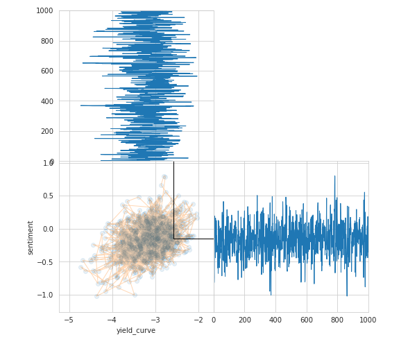
What should I interpret from this chart?
I also see there are two charts Metropolis-Hastings and NUTS but I’m not understanding the benefit or pros/cons of either method.
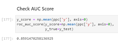
What should I derive from this AUC score? I see it’s from the test set data. Does it mean this model is 85% accurate at predicting a recession based on these variables?
Same question with the posterior predictive checks. What does this number represent?
In cell 13, we plot the mutual info between predictors and outcomes, where the recession outcome shifts 1-24 months into the future. The predictiveness ‘window’ varies by indicator. In cell 14, we shift the recession by 12 months, so we are trying to predict recessions 1 yr ahead.
The sample visualization just illustrates how the MCMC sampling process works. The models in this section are based on sampling and it’s important to understand how this works - we simultaneously pick values for different predictors and this needs to follow some empirical regularity. The little ‘movie’ shows how the algos draw samples for two of the four predictors. The mathematial details are a bit beyond the scope of the book but the pymc3 docs have more info. See pages 302-304 in the book for an overview.
For the pros and cons of Metropolis-Hastings and NUTS, see the excerpt below from the same location in the book that highlights several aspects and points out additional resources if you’d like to dive deeper.
The AUC score gives you the probability that two random samples are ranked correctly by the classifier. So 0.85 means there’s a 85% chance that if you pick two months where A is a recession and B is not that A has a higher score than B. This is different from accuracy and preferable because it accounts for class imbalances.
The section ‘Prediction’ illustrates how to make prediction and the intro briefly discusses how this works technically with ‘shared variables’. See the linked pymc3 docs for more detail…
The posterior predictive AUC score measures in-sample (training) performance.
Hope this helps!
Cheers, Stefan
Metropolis-Hastings sampling
The Metropolis-Hastings algorithm randomly proposes new locations based on its current state. It does so to effectively explore the sample space and reduce the correlation of samples relative to Gibbs sampling. To ensure that it samples from the posterior, it evaluates the proposal using the product of prior and likelihood, which is proportional to the posterior. It accepts with a probability that depends on the result relative to the corresponding value for the current sample.
A key benefit of the proposal evaluation method is that it works with a proportional rather than an exact evaluation of the posterior. However, it can take a long time to converge. This is because the random movements that are not related to the posterior can reduce the acceptance rate so that a large number of steps produces only a small number of (potentially correlated) samples. The acceptance rate can be tuned by reducing the variance of the proposal distribution, but the resulting smaller steps imply less exploration. See Chib and Greenberg (1995) for a detailed, introductory exposition of the algorithm.
Hamiltonian Monte Carlo – going NUTS
Hamiltonian Monte Carlo (HMC) is a hybrid method that leverages the first-order derivative information of the gradient of the likelihood. With this, it proposes new states for exploration and overcomes some of the MCMC challenges. In addition, it incorporates momentum to efficiently “jump around” the posterior. As a result, it converges faster to a high-dimensional target distribution than simpler random walk Metropolis or Gibbs sampling. See Betancourt (2018) for a comprehensive conceptual introduction.
The No U-Turn Sampler (NUTS, Hoffman and Gelman 2011) is a self-tuning HMC extension that adaptively regulates the size and number of moves around the posterior before selecting a proposal. It works well on high-dimensional and complex posterior distributions, and allows many complex models to be fit without specialized knowledge about the fitting algorithm itself. As we will see in the next section, it is the default sampler in PyMC3.