For:
We will build a SARIMAX model for monthly data on an industrial production time series for the 1988-2017 period. As illustrated in the first section on analytical tools, the data has been log-transformed, and we are using seasonal (lag-12) differences. We estimate the model for a range of both ordinary and conventional AR and MA parameters using a rolling window of 10 years of training data, and evaluate the RMSE of the 1-step-ahead forecast.
Finding the optimal number of lags
from joblib import Parallel, delayed
from tqdm import tqdm

train_size = 120  # 10 years of training data
test_set = industrial_production_log_diff.iloc[train_size:]

def fit_and_predict(params, train_size, industrial_production_log_diff):
    p1, q1, p2, q2 = params
    preds = test_set.copy().to_frame('y_true').assign(y_pred=np.nan)
    aic, bic = [], []
    if p1 == 0 and q1 == 0:
        return None
    convergence_error = stationarity_error = 0
    y_pred = []
    for i, T in enumerate(range(train_size, len(industrial_production_log_diff))):
        train_set = industrial_production_log_diff.iloc[T-train_size:T]
        try:
            with warnings.catch_warnings():
                warnings.filterwarnings("ignore")
                model = SARIMAX(endog=train_set.values,
                                order=(p1, 0, q1),
                                seasonal_order=(p2, 0, q2, 12)).fit(disp=0)
        except LinAlgError:
            convergence_error += 1
            continue
        except ValueError:
            stationarity_error += 1
            continue

        preds.iloc[i, 1] = model.forecast(steps=1)[0]
        aic.append(model.aic)
        bic.append(model.bic)

    preds.dropna(inplace=True)
    if preds.empty:
        return None

    mse = mean_squared_error(preds.y_true, preds.y_pred)
    return (p1, q1, p2, q2), [np.sqrt(mse),
                              preds.y_true.sub(preds.y_pred).pow(2).std(),
                              np.mean(aic),
                              np.std(aic),
                              np.mean(bic),
                              np.std(bic),
                              convergence_error,
                              stationarity_error]

# Parallel processing
results = Parallel(n_jobs=-1)(delayed(fit_and_predict)(params, train_size, industrial_production_log_diff) for params in tqdm(params))

# Filter out None results
results = {k: v for k, v in results if v is not None}
This version introduces parallel processing. 100% in ~14 minutes.
The following are some of the cells and their respective outputs just to show that the refactored code will not break anything that follows.
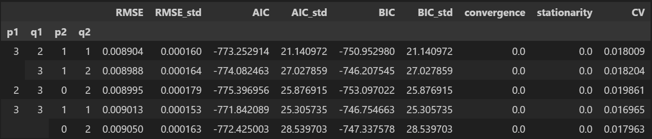
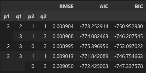
sarimax_results.nsmallest(5, columns='RMSE')
sarimax_results[['RMSE', 'AIC', 'BIC']].sort_values('RMSE').head()
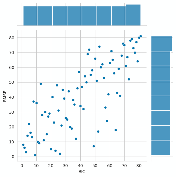
sns.jointplot(y='RMSE', x='BIC', data=sarimax_results[['RMSE', 'BIC']].rank());
.
.
.
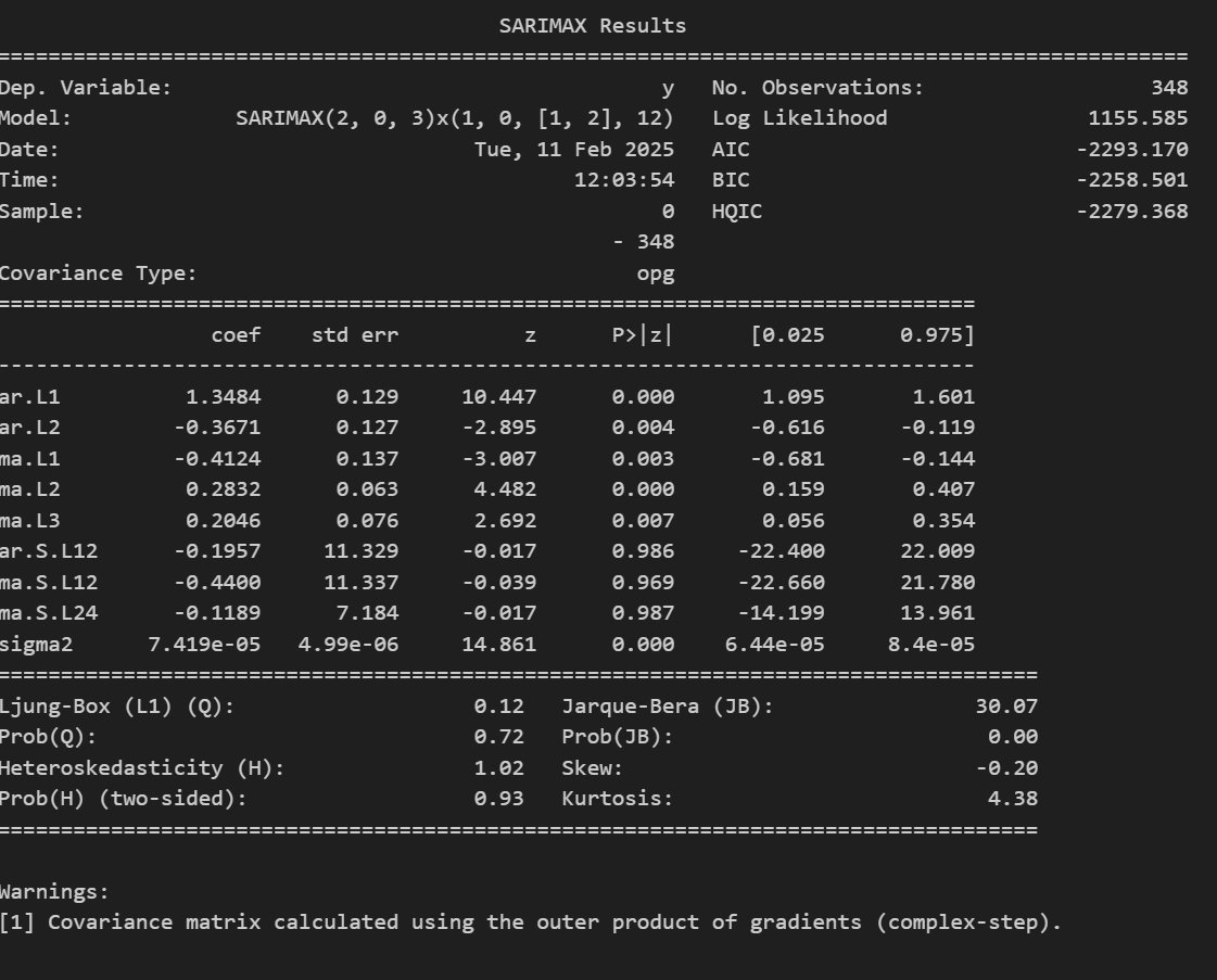
print(best_model.summary())
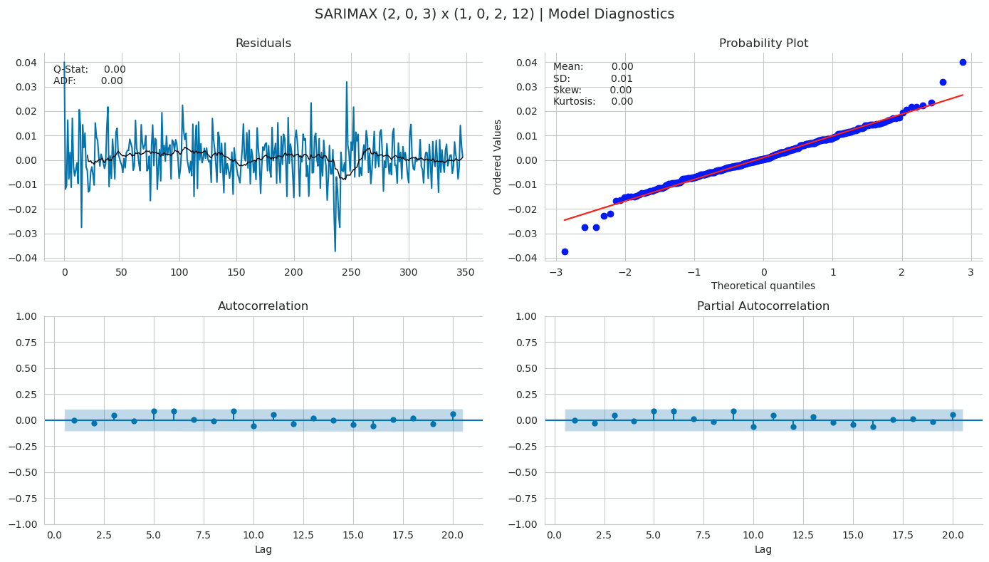
plot_correlogram(pd.Series(best_model.resid), lags=20, title=f'SARIMAX ({p1}, 0, {q1}) x ({p2}, 0, {q2}, 12) | Model Diagnostics')
Hope this helps.